How Models Work
预测,是机器学习的主要任务之一:利用training data,建立model进行fitting/training,最后对新的数据集进行predict。
Explore Your Data
我们使用pandas来查看并对数据集进行操作,如:
import pandas as pd
# read the data and store data in DataFrame
data = pd.read_csv(data_file_path)
# print a summary of the data in Melbourne data
data.describe()
describe()可以得到count, mean, std, min, max等信息。
Your First Machine Learning Model
一般地,把目标值设为y,特征值设为X。建立和使用模型主要有这么几步:1、选择一个合适的模型;2、利用训练集进行训练;3、对测试集的y进行预测;4、评价准确率等指标。
这里使用scikit-learn来建立机器学习模型,如:
from sklearn.tree import DecisionTreeRegressor
# Define model. Specify a number for random_state to ensure same results each run
model = DecisionTreeRegressor(random_state=1)
# Fit model
model.fit(X, y)
# Make predictions
predicted = model.predict(X)
Model Validation
模型学习效果的好坏总是需要适当的指标予以评价,比如MAE:
from sklearn.metrics import mean_absolute_error
predicted = model.predict(X)
mean_absolute_error(y, predicted)
模型是利用training data进行训练的,在其上使用评价指标缺乏泛化能力,并且易造成过拟合,我们需要validation data来反映模型的真实能力。
from sklearn.model_selection import train_test_split
train_X, val_X, train_y, val_y = train_test_split(X, y, random_state = 0)
melbourne_model = DecisionTreeRegressor()
model.fit(train_X, train_y)
val_predictions = model.predict(val_X)
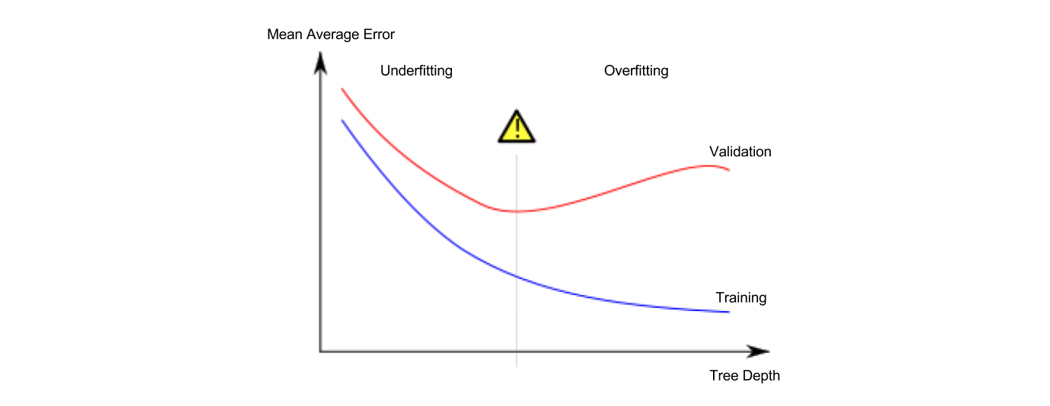
Underfitting and Overfitting
过拟合和欠拟合是常见的问题,这也是我们进行参数学习时重要的取舍指标。
# compare MAE with differing values of max_leaf_nodes
for max_leaf_nodes in [5, 50, 500, 5000]:
	my_mae = get_mae(max_leaf_nodes, train_X, val_X, train_y, val_y)
	print("Max leaf nodes: %d  \t\t Mean Absolute Error:  %d" %(max_leaf_nodes, my_mae))
Handling Missing Values
数据值缺失是实际应用中最常出现的问题。在python中,缺失的数值将用nan表示。
missing_val_count_by_column = (data.isnull().sum())
print(missing_val_count_by_column[missing_val_count_by_column > 0])
常见的一些解决办法有,1、将含有缺失值的特征值数列全部删除:
data_without_missing_values = original_data.dropna(axis=1)
# another way
cols_with_missing = [col for col in original_data.columns if original_data[col].isnull().any()]
reduced_original_data = original_data.drop(cols_with_missing, axis=1)
reduced_test_data = test_data.drop(cols_with_missing, axis=1)
2、缺失值插入:
from sklearn.impute import SimpleImputer
my_imputer = SimpleImputer()
data_with_imputed_values = my_imputer.fit_transform(original_data)
缺失值插入的办法一般要比直接删除的办法更准确,但插入什么样的值依然需要谨慎选择。另外,有的时候“缺失”本身也蕴含信息,把这些信息专门抽提出来也可能提高模型学习能力。
# make copy to avoid changing original data (when Imputing)
new_data = original_data.copy()
# make new columns indicating what will be imputed
cols_with_missing = [col for col in new_data.columns if new_data[col].isnull().any()]
for col in cols_with_missing:
	new_data[col + '_was_missing'] = new_data[col].isnull()
# Imputation
my_imputer = SimpleImputer()
new_data = pd.DataFrame(my_imputer.fit_transform(new_data))
new_data.columns = original_data.columns
Using Categorical Data with One Hot Encoding
离散型的分类数据不能简单地用函数曲线拟合,常见的处理方法之一是使用One-Hot Encoding,即将每一个离散变量作为一个新的特征编码。
one_hot_encoded_train = pd.get_dummies(train)
# Ensure the test data is encoded in the same manner as the training data with the align command
one_hot_encoded_train = pd.get_dummies(train)
one_hot_encoded_test = pd.get_dummies(test)
final_train, final_test = one_hot_encoded_train.align(one_hot_encoded_test, join='left', axis=1)
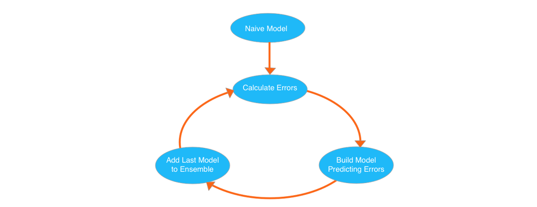
XGBoost
大拿模型,我的第一块Kaggle银牌。其核心算法是Gradient Boosted Decision Trees。
from xgboost import XGBRegressor
my_model = XGBRegressor()
my_model.fit(train_X, train_y, verbose=False)
predictions = my_model.predict(test_X)
from sklearn.metrics import mean_absolute_error
print("Mean Absolute Error : " + str(mean_absolute_error(predictions, test_y)))
XGBoost有一些参数需要优化调整(善于使用early_stopping_rounds将有助于调参),如n_estimators和learning_rate等:
my_model = XGBRegressor(n_estimators=1000, learning_rate=0.05)
my_model.fit(train_X, train_y, early_stopping_rounds=5, eval_set=[(test_X, test_y)], verbose=False)
Partial Dependence Plots
机器学习模型常被人诟病为黑箱子,你无法知道内部细节,无法得知各参数、各特征值对预测结果好坏的影响,其实我们完全可以使用部份依赖图来查看。
from sklearn.ensemble.partial_dependence import partial_dependence, plot_partial_dependence
# scikit-learn originally implemented partial dependence plots only for Gradient Boosting models
# this was due to an implementation detail, and a future release will support all model types.
my_model = GradientBoostingRegressor()
# fit the model as usual
my_model.fit(X, y)
# Here we make the plot
my_plots = plot_partial_dependence(my_model,
	features=[0, 2],			# column numbers of plots we want to show
	X=X,				# raw predictors data.
	feature_names=['A', 'B', 'C'], 	# labels on graphs
	grid_resolution=10) 		# number of values to plot on x axis
Pipelines
建立一个合适的流程才是王道,scikit-learn也提供了相应的模块:
from sklearn.ensemble import RandomForestRegressor
from sklearn.pipeline import make_pipeline
from sklearn.preprocessing import Imputer

my_pipeline = make_pipeline(Imputer(), RandomForestRegressor())
my_pipeline.fit(train_X, train_y)
predictions = my_pipeline.predict(test_X)
# Here is the code to do the same thing without pipelines
my_imputer = Imputer()
my_model = RandomForestRegressor()
imputed_train_X = my_imputer.fit_transform(train_X)
imputed_test_X = my_imputer.transform(test_X)
my_model.fit(imputed_train_X, train_y)
predictions = my_model.predict(imputed_test_X)
需要注意的是,scikit-learn的大部分对象是transformer或者model,在fit一个transformer后使用transform函数,在fit一个model后使用predict函数。pipeline必须从一个或多个transformer开始,由model结束。
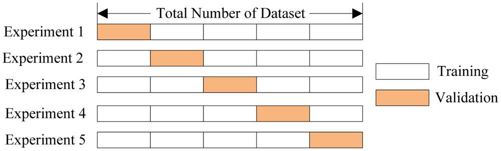
Cross-Validation
利用train_test_split分割出test是办法之一,但并不是最好的,毕竟依然存在随机性,分出多少数据也是问题,分出来了又造成数据浪费。在整体数据量不是特别大的时候,Cross-Validation不失为一个好办法:
 接着上一节的pipeline,这里有:
from sklearn.model_selection import cross_val_score
scores = cross_val_score(my_pipeline, X, y, scoring='neg_mean_absolute_error')
print(scores)
Data Leakage
机器学习中的数据泄露指的不是安全问题,而是模型沿着特定的数据分布做出了结果看起来很好,但不符合实际的预测。出现的原因比如有:将与结果直接相关的特征值纳入了数据集等。